Large Dataset Showcase

This page is the curated documentation version of dev/Untitled.ipynb. It keeps the same workflow on a real dataset, but adds context around grid construction, rasterization mode, and timing so the example is useful as a benchmark and not only as a screenshot.

What This Example Measures

The showcase uses a real building-footprint layer from a local GeoPackage:

Item	Value
Dataset	dev/data/BDT_3-5_GPKG_LAMB93_D075-ED2026-03-15.gpkg
Layer	batiment
Geometry count	606,667 polygons
CRS	EPSG:2154
Grid resolution	10 m
Grid shape	2,804 columns x 1,978 rows
Grid cells	5,546,312
Rasterization mode	area
GeoPackage read time	5.0 s
Measured rasterization time	13.1 s

The rasterization timing above corresponds to the compute step itself, separate from GeoPackage I/O. It was generated locally on a regular Windows 11 laptop with Python 3.13 and 16 logical CPUs using python scripts/generate_large_dataset_showcase.py, which also writes the committed image and metadata used by this page.

Notebook Flow

The original notebook starts with three steps: import the dependencies, load the building layer, and derive a regular Lambert-93 grid from the dataset bounds.

import geopandas as gpd
import numpy as np

from rasterizer import rasterize_polygons

gdf = gpd.read_file(
    "BDT_3-5_GPKG_LAMB93_D075-ED2026-03-15.gpkg",
    layer="batiment",
    columns=[],
)

xmin, ymin, xmax, ymax = gdf.total_bounds
resolution = 10.0
x = np.arange(xmin, xmax, resolution)
y = np.arange(ymin, ymax, resolution)

Using columns=[] keeps the example focused on geometry and avoids paying for unrelated attribute parsing when the goal is to benchmark rasterization throughput.

The actual computation is the same one-liner as in the notebook. The important point is that mode="area" returns the covered area of each cell in square meters because the input CRS is metric.

coverage = rasterize_polygons(
    polygons=gdf,
    x=x,
    y=y,
    crs=gdf.crs,
    mode="area",
)

Result

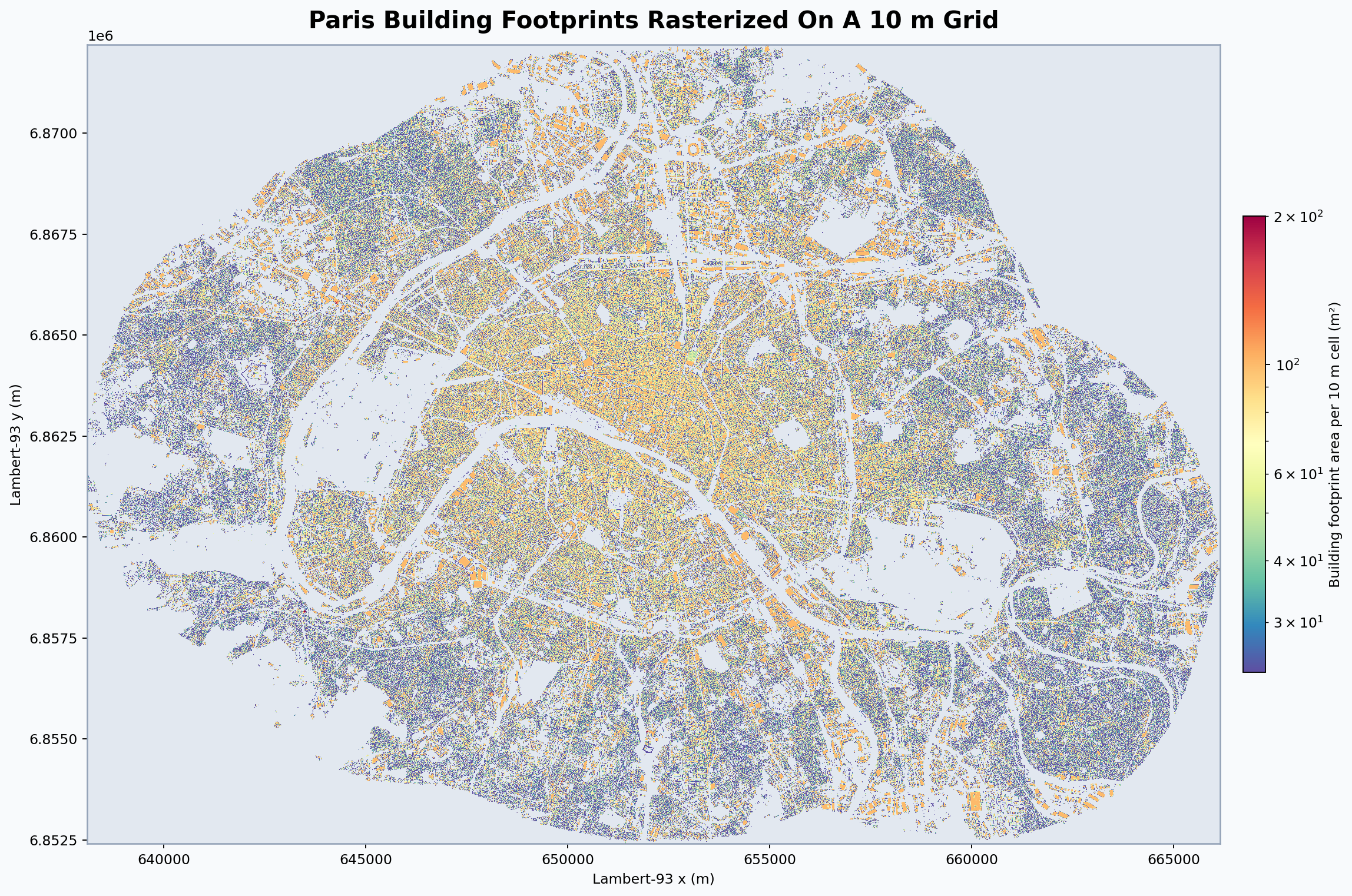
Building-footprint coverage rasterized on a regular 10 m Lambert-93 grid. Empty cells are muted and occupied cells use a logarithmic color scale so dense urban blocks remain readable.

The image is a good stress test for the package because it combines a large number of polygons with a grid large enough to matter, while still staying in the regular rectilinear case that rasterizer is designed to optimize.